Differential splicing and transcripts: Not as simple as it first appears
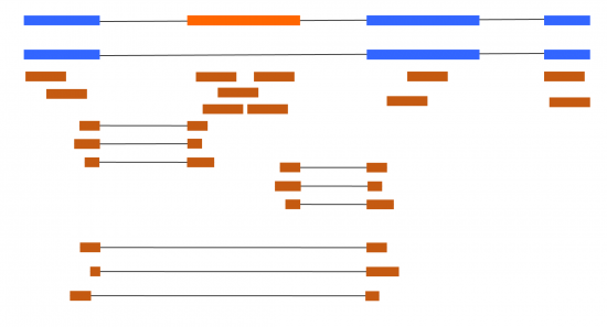
At first thought, dealing with alternative splicing with RNA-seq might appear simple. In the simplest situations, you could have a couple of different transcripts, and it is simple to work out if any increase from the reads mapping uniquely to each transcript (Figure 1).
Figure 1 – Blue boxes are constitutive exons, orange is an alternative (skipped) exon. Brown boxes are short reads from RNA-seq. Lines represent splice junctions (locations of intron removal).

However, the example in Figure 1 is very simplistic. A great textbook example, but does not convey the complexity of the splicing you will encounter when analyzing your own RNA-seq data. Transcripts are generally larger than three exons, involve multiple splicing events, some distant to each other, some overlapping. This can all make it diffecult to interpret what is going on. This post will discuss the multiple different approaches to dealing with alternative splicing and multiple transcript isoforms in your RNA-seq data and, suggest examples of different software designed to deal with this type of data.
This isn’t differential gene expression
Differential Gene Expression (DGE) is the most common thing RNA-seq data is used for. It can certainly be improved by taking into the multiple transcripts a gene produces to avoid certain artifacts (Cufflinks paper), but extra complications come into play if you want to focus on transcript rather than genes. When considering the simple example in Figure 1, with only one splicing event difference between the two transcripts, things are somewhat easy to analyze. But even then, we have multiple ways to analyze this data using fundamentally different approaches. The simplest way to example this would be to focus on the exon and its junctions in an exon-centric approach.
Exon-centric approach
Tools that take the exon-centric approach focus on individual junctions. Either the two junctions that correspond to skipped exon (or retained intron), or to the single junctions in alternative 5′ or 3′ splice site usage. This is a powerful approach. It directly informs us of the type of splicing event. We can simply count the number of reads that support the inclusion of an event (e.g. an exon inclusion) versus the number of reads that support the exclusion of an event (e.g. an exon skipping). The readout is a ratio: percentage spliced in (PSI). The higher this value, the more the exon is included in a sample. PSI is not a perfect, in the case of intron retention, the increase in PSI represents less splicing (i.e. the removal of the intron). Also, working with ratios does mean that the stats are not simple. Some of the tools developed for an exon-centric approach do not deal with replicates well. Some of the tools that take an exon-centric approach are:
rMATS
JUM
juncBASE
MISO
SUPPA*
*SUPPA actually uses transcript isoform data (see below) and produces both an exon-centric and isoform-centric output.
Isoform-centric
If instead we wanted to appreciate a transcript as a whole, rather than just the sum of its parts, we might want to take an isoform-centric approach. Transcript isoforms are often varied. A single gene can have MANY transcript isoforms with multiple splicing events generating this diversity (Figures 2 and 3).
Figure 2 – A third isoform is introduced compared to Figure 1. Lack of reads supporting it suggest that it might be an artefact in the annotation.

Many of these splicing events might be “complex”, depending on multiple co-regulation junctions (Figure 3). Isoform-centric approaches come in two flavors: Differential Transcript Expression (DTE) and Differential Transcript Usage (DTU). DTE is conceptually very simple for anyone who has done DGE before. DTE simply looks at what transcripts go up and down between two samples.
Figure 3 – Many transcript isoforms can exist per gene. Many events may appear to be co-spliced with distant events. When using standard short read data, it is impossible to know if these events are really co-regulated or if they just appear that way in the annotation, because a single short read cannot link the two together.

Tools like Salmon and Kallisto can quant transcript levels and these tools can be used to find differences between samples:
Sleuth
Ballgown
Despite DTE being conceptually easy to understand, it is probably the least useful for anyone interested in splicing. This is because a transcript isoform could increase in expression because of 1) changes in alternative splicing, 2) changes in transcription of the whole gene, leading to all/most isoforms increase or 3) both splicing and transcriptional changes.
Therefore, DTU might be more useful, because, as the name suggests, it focuses on the usage of transcript isoforms from the same gene, relative to each other. Therefore, DTU outputs as a ratio, like with PSI. However, rather than being a ratio of two states: inclusion and exclusion, DTU looks at the fraction each transcript takes up over all transcripts. If you have 10 transcript isoforms for a gene (not uncommon), you will have 10 ratios. This approach is useful as you can examine the change in proportion of a transcript between samples or over time. You can also better link the status of the whole transcript to its change. A transcript isoform might have particular features (UTR lengths, CDS length) that can be tricky to link with a single splicing event, especially when multiple splicing changes make that transcript what it is (Figure 3). DTU, compared to exon-centric approaches, lets you retain this information with a changing transcript. Some useful tools for DTU are:
RATs
SUPPA
One drawback to this approach compared to the exon-centric approaches is that you do not know which events are driving the splicing changes. For this, an exon-centric approach would be more useful. If embarking on a splicing focused project, it might be worth trying out a couple of different approaches and seeing which one gives you the most interpretable data for your particular problem. Each of the different approaches (exon-centric and isoform-centric) might reveal things that taking just one approach did not. Seeing features that appear in both might give you more confidence in your findings.
One last thing to consider
Another important thing to note is, how do we define the type of alternative splicing in reference to each other? If we look at our three transcript examples in Figure 2, we can see that the middle transcript could be defined as either an intron retained transcript or a alternative 3′ splice site (alternative acceptor site), depending on which of the two other transcripts you compare it too. If you compare it to the top transcript, the middle transcript looks just like an alternative 3′ splice site of the second exon. This is a very common form of splicing in plants after all. However, if you compare the middle isoform to the bottom one, then we see something completely different, we see that instead it appears to be a retained intron. Both interpretations are correct. The problem is, which one do you chose to annotate it as? Which one do you choose to quantify it as in an exon-centric approach? Each tool will have its own approach to dealing with situations like this. There is no easy answer. At this point I should mention that this is not simply a game of semantics, this has real biological consequences. To us, the interpretation of whether an event is a retained intron or an alternative 3′ splice site seems like a frustrating quirk of nomenclature that has no right answer, but to the cell, there are huge differences. For example, studies have shown that retained introns are not generally targeted to the RNA degradation pathway nonsense-mediated mRNA decay (NMD) in Arabidopsis, again in Arabidopsis and moss, and that they are actually often detained in the nucleus. So getting the annotation “right” in these cases does have huge implications in how to interpret your data. I do not have any good suggestions here, only please be aware of this potential issue and always look at some interesting splicing events in the genome browser to get a feel for what is really going on in your data – it is very tempting to purely rely on what a table is telling you is going on, but looking in the browser at the reads and transcript models can save you months of wasted time in analysis IMHO.
Here is a list of the software I have mentioned in this post. Please forgive me if I have missed off your favorite tool for splicing/isoform quant, this was not meant to be a comprehensive list but instead an introduction to the topic. Please feel free to discuss what are your personal favorite tools in the comments below.
- rMATS:
http://www.pnas.org/content/11… - JUM:
http://www.pnas.org/content/11… - juncBASE:
https://github.com/anbrooks/ju… - MISO:
https://www.nature.com/article… - SUPPA:
https://genomebiology.biomedce… - Salmon:
https://www.nature.com/article… - Kallisto:
https://www.nature.com/article… - Sleuth:
https://www.nature.com/article… - Ballgown:
https://www.nature.com/article… - RATs:
https://www.biorxiv.org/conten…
Finally, please check out my blog, Bad Grammar Good Syntax. It offers an introduction to computational biology for those with less of a programming background. It has great posts on particular topics such as understanding basic terms in RNA-seq, making good Venn diagrams with Python, using UpSets instead of Venn diagrams for multiple set overlaps, and how to install Ubuntu on Windows 10 for computational biology.


Leave a Reply
Want to join the discussion?Feel free to contribute!